Best Popcorn

One hundred shoppers in a grocery store each tasted three brands of popcorn and rated each one from 1 (awful) to 10 (amazing). Which brand is best, and is the difference big enough to be more than chance?

This walkthrough answers that question entirely in the SciStack GUI. In the Code version, you wrote a function for each step: importing the data, summarising each brand, and running each test. Here you write no code at all. The canvas imports the CSV into a database, Plot Studio draws the figure, and Stat Studio runs the statistics. Each step explains why as well as what, so you can apply the same reasoning to your own data.

What you'll learn

• How to choose a schema for a real dataset, and why its names matter.
• How to import a CSV on the canvas with a library function, so each row becomes its own record.
• How to turn one of a function's default settings into a Parameter that anyone can change.
• How roles in Plot Studio turn the same data into different figures.
• How Stat Studio picks the right statistical test from your study's design, and when to choose differently.
• How a figure and its statistics stay linked.

Before you start, install the VS Code extension and the scistack package.

The data

The dataset has 300 rows: 100 participants × 3 brands. It's in long format, meaning one row per rating:

participant	brand	rating
P001	Butterburst	5
P001	KettleKing	5
P001	SeaSaltCo	4
P002	Butterburst	7
…	…	…

Download: popcorn_ratings.csv

If the download doesn't work for you, expand the box below, copy the contents (the copy button is in the top-right corner of the code block), and save them as popcorn_ratings.csv.

popcorn_ratings.csv (click to expand)

type: example

participant,brand,rating
P001,Butterburst,5
P001,KettleKing,5
P001,SeaSaltCo,4
P002,Butterburst,7
P002,KettleKing,7
P002,SeaSaltCo,6
P003,Butterburst,8
P003,KettleKing,6
P003,SeaSaltCo,6
P004,Butterburst,7
P004,KettleKing,8
P004,SeaSaltCo,8
P005,Butterburst,6
P005,KettleKing,6
P005,SeaSaltCo,6
P006,Butterburst,5
P006,KettleKing,7
P006,SeaSaltCo,4
P007,Butterburst,9
P007,KettleKing,9
P007,SeaSaltCo,8
P008,Butterburst,9
P008,KettleKing,6
P008,SeaSaltCo,4
P009,Butterburst,8
P009,KettleKing,8
P009,SeaSaltCo,3
P010,Butterburst,10
P010,KettleKing,8
P010,SeaSaltCo,8
P011,Butterburst,8
P011,KettleKing,5
P011,SeaSaltCo,3
P012,Butterburst,9
P012,KettleKing,10
P012,SeaSaltCo,8
P013,Butterburst,10
P013,KettleKing,7
P013,SeaSaltCo,5
P014,Butterburst,8
P014,KettleKing,9
P014,SeaSaltCo,4
P015,Butterburst,8
P015,KettleKing,8
P015,SeaSaltCo,6
P016,Butterburst,7
P016,KettleKing,6
P016,SeaSaltCo,5
P017,Butterburst,9
P017,KettleKing,9
P017,SeaSaltCo,8
P018,Butterburst,8
P018,KettleKing,8
P018,SeaSaltCo,8
P019,Butterburst,8
P019,KettleKing,5
P019,SeaSaltCo,3
P020,Butterburst,5
P020,KettleKing,6
P020,SeaSaltCo,5
P021,Butterburst,9
P021,KettleKing,7
P021,SeaSaltCo,6
P022,Butterburst,8
P022,KettleKing,8
P022,SeaSaltCo,5
P023,Butterburst,6
P023,KettleKing,4
P023,SeaSaltCo,3
P024,Butterburst,6
P024,KettleKing,5
P024,SeaSaltCo,3
P025,Butterburst,8
P025,KettleKing,6
P025,SeaSaltCo,5
P026,Butterburst,10
P026,KettleKing,5
P026,SeaSaltCo,7
P027,Butterburst,6
P027,KettleKing,6
P027,SeaSaltCo,6
P028,Butterburst,8
P028,KettleKing,8
P028,SeaSaltCo,9
P029,Butterburst,9
P029,KettleKing,5
P029,SeaSaltCo,6
P030,Butterburst,5
P030,KettleKing,6
P030,SeaSaltCo,5
P031,Butterburst,8
P031,KettleKing,9
P031,SeaSaltCo,5
P032,Butterburst,7
P032,KettleKing,6
P032,SeaSaltCo,7
P033,Butterburst,3
P033,KettleKing,6
P033,SeaSaltCo,5
P034,Butterburst,10
P034,KettleKing,9
P034,SeaSaltCo,6
P035,Butterburst,8
P035,KettleKing,6
P035,SeaSaltCo,8
P036,Butterburst,10
P036,KettleKing,9
P036,SeaSaltCo,7
P037,Butterburst,5
P037,KettleKing,3
P037,SeaSaltCo,6
P038,Butterburst,10
P038,KettleKing,8
P038,SeaSaltCo,7
P039,Butterburst,9
P039,KettleKing,9
P039,SeaSaltCo,7
P040,Butterburst,8
P040,KettleKing,8
P040,SeaSaltCo,6
P041,Butterburst,6
P041,KettleKing,6
P041,SeaSaltCo,4
P042,Butterburst,5
P042,KettleKing,5
P042,SeaSaltCo,4
P043,Butterburst,5
P043,KettleKing,7
P043,SeaSaltCo,5
P044,Butterburst,4
P044,KettleKing,6
P044,SeaSaltCo,2
P045,Butterburst,5
P045,KettleKing,7
P045,SeaSaltCo,4
P046,Butterburst,7
P046,KettleKing,5
P046,SeaSaltCo,6
P047,Butterburst,9
P047,KettleKing,5
P047,SeaSaltCo,5
P048,Butterburst,6
P048,KettleKing,7
P048,SeaSaltCo,7
P049,Butterburst,5
P049,KettleKing,5
P049,SeaSaltCo,5
P050,Butterburst,8
P050,KettleKing,5
P050,SeaSaltCo,6
P051,Butterburst,8
P051,KettleKing,9
P051,SeaSaltCo,6
P052,Butterburst,7
P052,KettleKing,7
P052,SeaSaltCo,6
P053,Butterburst,6
P053,KettleKing,5
P053,SeaSaltCo,6
P054,Butterburst,5
P054,KettleKing,6
P054,SeaSaltCo,6
P055,Butterburst,7
P055,KettleKing,5
P055,SeaSaltCo,3
P056,Butterburst,10
P056,KettleKing,8
P056,SeaSaltCo,9
P057,Butterburst,6
P057,KettleKing,6
P057,SeaSaltCo,3
P058,Butterburst,8
P058,KettleKing,7
P058,SeaSaltCo,8
P059,Butterburst,10
P059,KettleKing,9
P059,SeaSaltCo,7
P060,Butterburst,10
P060,KettleKing,5
P060,SeaSaltCo,3
P061,Butterburst,9
P061,KettleKing,9
P061,SeaSaltCo,7
P062,Butterburst,6
P062,KettleKing,6
P062,SeaSaltCo,5
P063,Butterburst,9
P063,KettleKing,8
P063,SeaSaltCo,6
P064,Butterburst,10
P064,KettleKing,5
P064,SeaSaltCo,5
P065,Butterburst,8
P065,KettleKing,5
P065,SeaSaltCo,5
P066,Butterburst,9
P066,KettleKing,7
P066,SeaSaltCo,7
P067,Butterburst,8
P067,KettleKing,7
P067,SeaSaltCo,8
P068,Butterburst,8
P068,KettleKing,7
P068,SeaSaltCo,3
P069,Butterburst,7
P069,KettleKing,6
P069,SeaSaltCo,5
P070,Butterburst,6
P070,KettleKing,6
P070,SeaSaltCo,4
P071,Butterburst,4
P071,KettleKing,6
P071,SeaSaltCo,5
P072,Butterburst,7
P072,KettleKing,7
P072,SeaSaltCo,6
P073,Butterburst,5
P073,KettleKing,6
P073,SeaSaltCo,6
P074,Butterburst,7
P074,KettleKing,5
P074,SeaSaltCo,6
P075,Butterburst,7
P075,KettleKing,6
P075,SeaSaltCo,5
P076,Butterburst,9
P076,KettleKing,9
P076,SeaSaltCo,9
P077,Butterburst,7
P077,KettleKing,7
P077,SeaSaltCo,2
P078,Butterburst,10
P078,KettleKing,7
P078,SeaSaltCo,9
P079,Butterburst,7
P079,KettleKing,6
P079,SeaSaltCo,7
P080,Butterburst,4
P080,KettleKing,4
P080,SeaSaltCo,2
P081,Butterburst,6
P081,KettleKing,4
P081,SeaSaltCo,3
P082,Butterburst,5
P082,KettleKing,2
P082,SeaSaltCo,3
P083,Butterburst,9
P083,KettleKing,5
P083,SeaSaltCo,5
P084,Butterburst,7
P084,KettleKing,6
P084,SeaSaltCo,4
P085,Butterburst,6
P085,KettleKing,4
P085,SeaSaltCo,7
P086,Butterburst,6
P086,KettleKing,6
P086,SeaSaltCo,5
P087,Butterburst,7
P087,KettleKing,8
P087,SeaSaltCo,5
P088,Butterburst,8
P088,KettleKing,6
P088,SeaSaltCo,6
P089,Butterburst,10
P089,KettleKing,5
P089,SeaSaltCo,4
P090,Butterburst,6
P090,KettleKing,3
P090,SeaSaltCo,2
P091,Butterburst,10
P091,KettleKing,8
P091,SeaSaltCo,6
P092,Butterburst,4
P092,KettleKing,4
P092,SeaSaltCo,5
P093,Butterburst,4
P093,KettleKing,1
P093,SeaSaltCo,4
P094,Butterburst,7
P094,KettleKing,6
P094,SeaSaltCo,7
P095,Butterburst,6
P095,KettleKing,6
P095,SeaSaltCo,6
P096,Butterburst,8
P096,KettleKing,6
P096,SeaSaltCo,6
P097,Butterburst,10
P097,KettleKing,4
P097,SeaSaltCo,4
P098,Butterburst,5
P098,KettleKing,7
P098,SeaSaltCo,6
P099,Butterburst,7
P099,KettleKing,5
P099,SeaSaltCo,5
P100,Butterburst,8
P100,KettleKing,9
P100,SeaSaltCo,7

Step 1: Set up a folder

Make a new folder called best-popcorn, with a data folder inside it, and put popcorn_ratings.csv in data:

best-popcorn/
└── data/
    └── popcorn_ratings.csv

Open the best-popcorn folder in VS Code (File > Open Folder…). SciStack treats the open folder as your project, and everything it creates goes inside it.

Step 2: Create the database and choose the schema

Run SciStack: Open Pipeline from the Command Palette and choose to create a new database. SciStack asks where to put it: select the best-popcorn folder and click Select Folder.

Then name the database best-popcorn and press Enter.

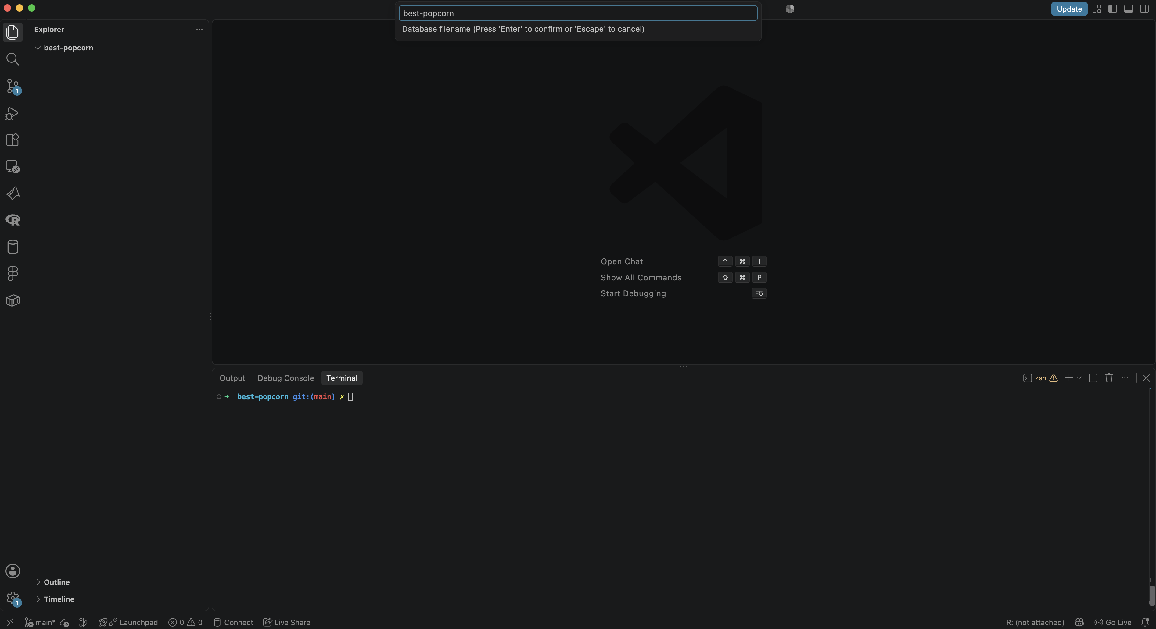
Next, SciStack asks for your schema keys. The schema describes how the dataset is organised: the things that identify each rating. Here, each rating is identified by who gave it and which brand it's for, so enter:

participant, brand

rating isn't part of the schema. It's the value that was measured, not part of how the data is organised.

Use the CSV's column names exactly

When SciStack imports a table, it looks for columns named after your schema keys to work out where each row belongs. Name the keys participant and brand, matching the CSV's column headers exactly. If you used person instead of participant, SciStack wouldn't recognise the participant column, and the ratings would be filed in the wrong places.

You now have a blank canvas. SciStack has also created a few files in the folder: the database (best-popcorn.duckdb), a settings file (scistack.toml), and a src folder for any code you add later. The database holds your data and the record of how every result was made.

Step 3: Point SciStack at the CSV

The first job is to get the ratings into the database. Start by telling SciStack where the file is.

In the sidebar, open the Path Inputs tab (📁), click +, and name the new path input data. Click it, and in its settings set the Path Template to:

data/popcorn_ratings.csv

Drag data from the sidebar onto the canvas.

A path input can contain schema keys in curly braces, such as data/{participant}.csv, when the data is split across one file per participant. This dataset is all in one file, so the template is just the path.

Step 4: Add a function to read it

Reading a CSV is a solved problem, so there's no need to write a function for it. Use pandas' read_csv.

Open the Functions tab (f(x)), click +, and enter pandas.read_csv. Drag it onto the canvas.

Now connect them: drag from the handle on data to read_csv's first input, filepath_or_buffer. The arrow says that this function reads this file.

Why not just open the file?

Running the import through the canvas means SciStack records that the ratings came from popcorn_ratings.csv, read by pandas.read_csv. Every result you calculate later can be traced back to this file.

read_csv has dozens of other settings, all with defaults, so the node only shows the one it needs. One of them is worth making visible: the separator between columns. Your file uses commas, which is read_csv's default, but a spreadsheet saved in many European languages uses semicolons. Making it a Parameter records which one was used, and lets anyone who gets this project change it without touching code (you'll see that in Step 14).

1. Open the Parameters tab (P), click +, and name the new parameter SEP.
2. Under Add value, type a single comma, ,, and click Add.
3. Drag SEP onto the canvas.
4. Drag from SEP's handle onto ＋ argument under read_csv's name. A list of read_csv's other settings opens, each with its default. Type sep and choose sep = ','.

read_csv now has a second input, sep, connected to SEP. It still reads the file exactly as before, because , is what it used anyway.

📷 Screenshot

Show: data → read_csv (filepath_or_buffer) and SEP → read_csv (sep), with the ＋ argument list closed and the Parameters tab showing SEP with the value ,. Save as docs/images/example_best-popcorn/connect_sep_parameter.png.

Step 5: Create the Rating variable

A variable is a named kind of data that the database stores, such as "a rating". Open the Variables tab (x), click +, and name it Rating. Drag it onto the canvas, then connect read_csv's output to it.

The read_csv node is red. That's expected: red means the step has no results yet. It turns green once it has run.

Step 6: Run the import

Click ▶ Run on the read_csv node.

Here's what happens:

1. read_csv runs once and returns the whole 300-row table. It runs once because the path input points at a single file.
2. SciStack sees that the table has participant and brand columns, which match your schema keys, so it treats each row as its own record. The row P001, Butterburst, 5 is saved as a Rating of 5 at participant = P001, brand = Butterburst.
3. The node turns green, and the Runs dock reports the run as finished.

Check the result: right-click Rating and choose View Schema Locations. The dialog should say 300/300 locations green: all 100 participants × 3 brands have a rating.

From here on, nothing reads the CSV again. Every later step reads Rating from the database.

Step 7: Look at the raw data

Click Rating, then Open Plot Studio → in the sidebar. Plot Studio opens in a new tab.

Look at the Structure group in the left rail. Plot Studio has put brand in Grouping, so there's one mark per brand. participant is set to Separate figures, so there's one figure per participant. Use ◀ and ▶ above the figure to step through them: P001, P002, and so on. The counter beside them shows which of the 100 you're on.

This is a good habit: look at individual data before averaging it. A participant who rated every brand 10, or a typo such as a rating of 55, is easy to spot here and hard to spot in an average.

Step 8: Summarise each brand in a figure

To compare the brands across everyone, average over the participants. In Structure > Factors, change participant from Separate figures to Average over.

There's now a single figure, with each brand summarising all 100 participants. Then:

1. In Chart, choose Bar + error.

2. In Statistics > Summary, set Centre to Mean and Spread to SD.

   

3. In Statistics > Show sample, tick participant and leave Join points on Auto (lines).

The lines are worth a moment. Each line is one participant, joining their three ratings. This shows the study's most important feature: every person rated every brand. Because of that, the fair comparison is within each person, as in "did this person prefer Butterburst to KettleKing?", rather than between the three bars as if they were separate groups of people. Keep that in mind for the statistics.

To tell the participants apart, set Colour points by to participant, which gives each person's line its own colour.

The means are about 7.3 for Butterburst, 6.3 for KettleKing and 5.5 for SeaSaltCo. Butterburst looks best, but is the difference more than chance?

Before moving on, save the figure. In the Saved plots rail on the right, name it Ratings by brand and save it. Saving it lets the statistics link to it in the next step. Use Save image in the toolbar if you want a file for a slide.

Step 9: Describe the study to Stat Studio

Click StatStudio in Plot Studio's toolbar. Stat Studio opens in a new tab, already set up from the figure: Rating as the measure, brand grouped, and participant collapsed.

A new table opens in the Step by step view. Each screen asks one question, shows what Stat Studio found in your data, and recommends an answer. What does this mean? explains any idea a screen names. Press Next → to go on, or ← Back to change an earlier answer. The first five screens describe the study:

• What did you measure? Rating: 300 values from 100 participants.

  

• What is one independent thing you measured? Each participant counts once: 100 participants in total. This is the most important question in statistics. Each person's three ratings belong together. A test that treated 300 ratings as 300 separate people would be far too sure of itself.

  

• What are you comparing? brand is set to Compare, and participant to Average over. These are the roles from Plot Studio, in Stat Studio's words.

  

• Was each participant measured at every level? Stat Studio recommends Same participants, measured repeatedly, because each of the 100 participants rated every brand. This is what the lines in the figure showed.

  

• Is anything missing? Every participant was measured at every level. Nothing to decide.

  

Step 10: Choose the test

The next screens choose and run the tests.

• What is your main question? Every pair of brands, which is 3 comparisons. Keep Yes, an overall test and then the pairs: first ask whether the brands differ at all, then which pairs differ.

  

• Which test? Stat Studio checks the shape of the data and finds that the values are roughly bell-shaped, so it recommends a paired t-test for the pairs and an ANOVA overall, and selects them for you. Keep them.

  

  Both are paired: the paired t-test compares each person's own two ratings, and the ANOVA treats brand as measured within each participant. Tests for separate groups of people, such as Welch's t-test and the Mann–Whitney U test, are greyed out, and each one says why underneath: brand is within.

Ratings are ranks

A 1–10 taste score is a ranking, not a physical measurement: a 6 is better than a 5, but the step from 5 to 6 isn't guaranteed to equal the step from 9 to 10. Tests based on ranks don't assume equal steps. If you'd rather not assume them either, choose Wilcoxon signed-rank test under Comparing pairs and Friedman test under Overall test. For this data the conclusion is the same.

• How should false alarms be kept rare? Three comparisons mean three chances of a fluke. Keep the recommended Holm correction, which adjusts the p values for that.

  

• How should the size of each difference be reported? For a paired t-test, Stat Studio recommends Cohen's d_z: the average difference divided by how much the differences vary between people. Keep it, and keep the 95% CI of the difference for the uncertainty.

  

Step 11: Read the results

• Your results. 3 of 3 comparisons ran; 3 significant at α = 0.05 after the correction.

  

The pairs come first, under Comparisons:

Comparison	Δ [95% CI]	Statistic	p (adj.)	Cohen's d_z
Butterburst − KettleKing	0.95 [0.59, 1.31]	t(99) = 5.28	< .001	0.53 [0.32, 0.74]
Butterburst − SeaSaltCo	1.82 [1.44, 2.20]	t(99) = 9.53	< .001	0.95
KettleKing − SeaSaltCo	0.87 [0.54, 1.20]	t(99) = 5.22	< .001	0.52

Butterburst is rated higher than both other brands, by about one point over KettleKing and nearly two over SeaSaltCo. Each row gives the difference with its direction (Butterburst − KettleKing), its confidence interval, the test statistic, and the effect size. The note under the table records everything a reader needs to know, such as the tests, the unit, n and the correction, and also the checks the tests relied on, such as a Shapiro–Wilk normality check of each pair's differences.

The overall test is under Omnibus: the ANOVA gives F(2.0, 193.4) = 51.44, p < .001, generalised η² = 0.16. The brands are not equally liked. The note under it says the degrees of freedom are Greenhouse–Geisser corrected (ε = 0.98), a small adjustment that repeated-measures ANOVA makes when the brands' differences vary unevenly.

Under the tables, Results as sentences writes the same findings in words. Click Copy sentences to start your results section. The Rating by brand table below it shows each brand's mean (SD): 7.3 (1.8), 6.3 (1.7) and 5.5 (1.7). To put a table in a paper, choose html and click Copy. It pastes into Word as a formatted table, with its note.

A small difference from the Code version

The Code version used rank-based tests (Friedman overall, then Wilcoxon), compared the best brand with each of the other two, and used a Bonferroni correction. Here Stat Studio uses its recommended paired t-tests and ANOVA, compares every pair (including KettleKing against SeaSaltCo), and uses Holm, which is slightly less strict but still guards against flukes across all three comparisons. The conclusion is the same. To match the Code version, choose Wilcoxon signed-rank test and Friedman test on the "Which test?" screen and Bonferroni correction on the false-alarms screen.

Name the table Popcorn statistics and save it.

Step 12: Put the result on the figure

Click Advanced at the top of Stat Studio. It shows every setting at once, including the answers you just gave. Under Brackets on the figure, tick Draw test brackets on the linked figure, keep Pairs on the significant ones and Label on stars, and save the table again.

Switch back to the Plot Studio tab. Ratings by brand now has brackets between the brands that differ, drawn from the test results rather than typed by hand. If the data or the test settings change, the brackets follow.

Step 13 (optional): Make it part of the pipeline

So far, the figure and the table are saved views of the data. To make them steps in the pipeline, click Add to pipeline: in Plot Studio's toolbar for the figure, and in Stat Studio for the table. Each one appears on the canvas, connected to Rating.

The difference is that pipeline steps are recorded like any other result. If the ratings change, they turn red until you re-run them, and 📄 Report collects them into a single web page with a note of where each came from.

Step 14 (optional): Share the project with a colleague

Suppose a colleague at another store ran the same taste test and wants to analyse it the same way. You send them the whole project as one file. They import it, point it at their own CSV, and re-run it. They write no code either.

Their data differs from yours in three ways, all common in practice:

• Their CSV calls the people shopper, not participant: the columns are shopper, brand, rating.
• The file is called store2_ratings.csv, and it sits in a folder of their own, popcorn-store2/.
• Their spreadsheet program saved it with semicolons between the columns (shopper;brand;rating), as Excel does in many European languages.

What you do: export

1. Check the dependencies. The project's only code is pandas.read_csv, and pandas comes with SciStack, so pyproject.toml needs nothing more. In your own projects, add every package your code imports (see Before you export).
2. Click ⇩ export project at the right end of the hypothesis tab strip.
3. Choose what goes in besides the code, settings and canvas:
   • History: tick it. It costs little and lets anyone check the results later.
   • Data: leave it off. Your colleague will run the pipeline on their own ratings, so they don't need your results.
   • Wheelhouse: leave it off. It's only for libraries, and this project uses none.
4. Click Export… and save best-popcorn.scistack. Send it to your colleague.

The file holds the canvas, the data path input, the SEP Parameter with its value, the Rating variable, the saved figure Ratings by brand and the saved table Popcorn statistics. It does not hold popcorn_ratings.csv: raw data files never travel. Send the CSV separately if your colleague should reproduce your results too (see Reproducing your results below).

What your colleague does: import

They need VS Code, the SciStack extension and a virtual environment with SciStack installed (New to Coding? steps 4 and 7). Then:

1. Open the Command Palette (View → Command Palette…), run SciStack: Import Project Bundle… and pick best-popcorn.scistack.
2. Where should the new project go? Pick a parent folder, then accept the folder name best_popcorn or type another, such as best-popcorn-store2. An import always creates a new folder.

3. Your schema keys. The box suggests yours, participant, brand. Their CSV says shopper, so they change it to:

   shopper, brand
   

   The keys must match the CSV's column headers, for the same reason as in Step 2.

4. The exporter's key "participant" is not in your schema. Which of your keys is "participant"? They pick shopper. SciStack now renames participant to shopper everywhere the project mentions it: in the saved figure's roles (collapse participant, show sample participant, colour points by participant) and in the saved table's design (average over participant). If a key has no counterpart at all, choose (drop it — no counterpart in my schema), and anything that mentions it is removed and listed in the report.

5. PathInput "data": data/popcorn_ratings.csv. Raw files aren't in the bundle, so SciStack asks where theirs are:
   • Choose my folder…: pick the folder the template is read from. They choose popcorn-store2/.
   • Keep the exporter's folder: only useful on the same computer.
   • Decide later (edit the entities file): set it in the sidebar after opening.
6. History. Choose Skip history. With a changed schema, your history couldn't be loaded into their database anyway (it describes participants, not shoppers), and their results will come from their own data.
7. The import report opens as a document. Under Schema keys it shows participant → shopper. Under Review it lists the saved figure and the saved table, because both mentioned participant: worth a look once the data is in.
8. Click Trust, Install and Open. SciStack installs any packages the project needs that are missing, at your versions, and opens the project. (Trust and Open opens it without installing anything.) Both buttons mean "I trust this file": opening a project runs its code, so only do this with files from people you trust.

📷 Screenshot

Show: the Which of your keys is "participant"? picker with shopper highlighted, and the import report beside it showing participant → shopper and two items under Review.

What your colleague changes after opening

The canvas looks like yours: data and SEP → read_csv → Rating, all red, because nothing has run in this project yet. The schema above the canvas reads schema: [shopper, brand].

The path input. The file name is still yours. In the Path Inputs tab (📁), click data and change its Path Template to:

store2_ratings.csv

The root folder, popcorn-store2/, was set during the import, so the template is the path within it. If they chose Decide later, set the root folder here too.

The separator. Their spreadsheet program saved the file with semicolons between the columns, not commas. With SEP still ,, read_csv would read each whole line as a single column, so there would be no shopper or brand column to file the ratings by. Open the Parameters tab (P) and click SEP. It arrived with your value, ,. Click × next to , to remove it, then type ; under Add value and click Add.

Remove the old value rather than keeping both: a Parameter with two values runs its step once for each, and the , run would read this file wrongly. Their values are theirs alone: nothing they change reaches your project, and nothing you change later reaches theirs.

Run it. Click ▶ Run on read_csv. Right-click Rating and choose View Schema Locations to check that every shopper has a rating for every brand.

Check the figure and the table. Click Rating, then Open Plot Studio →. Pick Ratings by brand from the Saved plots rail: it's drawn from their ratings, with shopper collapsed where you had participant. Open StatStudio from the toolbar and click Popcorn statistics under the saved tables. Step through the screens once: the answers came from your study, so confirm they still hold for theirs (each shopper rated every brand, nothing is missing) before reading the results.

📷 Screenshot

Show: the colleague's canvas after the run, all green, with schema: [shopper, brand] above it, and the Path Inputs tab open on data with the template store2_ratings.csv, or the Parameters tab open on SEP with the value ;.

Reproducing your results

To check your analysis rather than extend it, your colleague needs your CSV too. They import the same way, with three differences:

• At Your schema keys, they keep participant, brand. No key question follows.
• At PathInput "data", they choose the folder that holds data/popcorn_ratings.csv. The template stays as it is.
• At History, they choose Import history.

After Run all, they click ✓ verify in the hypothesis tab strip. It runs nothing: it compares their results with the history you exported, step by step, and should report every step as reproduced. Any difference is listed at the step where it first appears.

See Export & Import Projects for every option.

Summary

Here's how the same analysis looks in code and in the GUI:

	Code (scidb)	GUI
Setup	configure_database("popcorn.duckdb", ["participant", "brand"])	SciStack: Open Pipeline, schema keys participant, brand
Import	A load_ratings function, run with for_each	A path input and a SEP Parameter wired into pandas.read_csv, wired into Rating
Summary per brand	A summarize_ratings function, run once per brand	Plot Studio: brand grouped, participant collapsed
Overall test	A friedman_test function	Stat Studio Step by step: within-subject from the design; the recommended repeated-measures ANOVA
Which is best	A compare_to_best function, Wilcoxon, Bonferroni	Stat Studio pairwise paired t-tests, Holm
Afterwards	load(...) any result; get_provenance	Saved plot and saved table; Add to pipeline for recorded steps
Sharing	scistack export / scistack import / scistack verify	⇩ export project; SciStack: Import Project Bundle…; ✓ verify

Conclusion

The analysis supports a write-up like this:

Taste ratings differed across the three brands (repeated-measures ANOVA, Greenhouse–Geisser corrected: F(2.0, 193.4) = 51.4, p < 0.001, generalised η² = 0.16). Butterburst (mean 7.3/10) was rated higher than both KettleKing (mean 6.3; Δ = 0.95, 95% CI [0.59, 1.31], d_z = 0.53) and SeaSaltCo (mean 5.5; Δ = 1.82, 95% CI [1.44, 2.20], d_z = 0.95; paired t-tests, Holm-adjusted p < 0.001 for both).

Butterburst is the best popcorn.

Where to go next

• Process, Visualize and Summarize describe each part of the GUI in more detail.
• Best Player: a second example, with missing data, leaving a player out, and statistics on groups of different people.